How to get the most from the Curvefitter
Note: Examples provided by TCI Corp.
Understanding the Curvefitter processor and how to adjust it will produce the most ideal results.
What does the plug-in do?
The FME Curvefitter plug-in smooths lines derived from line segments, points or raster data, and replaces a series of line segments with the optimal combination of straight lines and embedded arc segments required to create smooth curving lines.
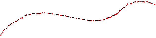
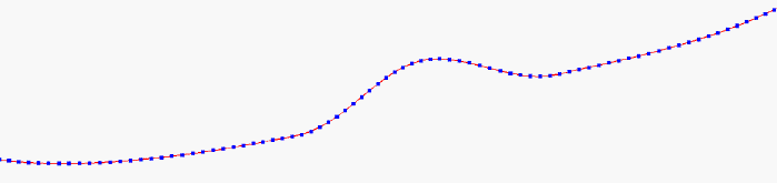
Example 1: This simple linestring could have been extracted from any FME-supported format. It’s made up of 85 straight line segments.
The Ideal Solution
The ideal solution for any Curvefitter process will depend on:
- the characteristics of the source linework
- the goals of the operator.
For this example, we will assume the linework represents an engineered feature such as a road ROW boundary. As such, the linework was probably originally defined by Arcs and Lines. Our goal is to create linework that recreates that structure while accurately fitting the original linework. With these assumptions, our “Ideal Solution” will contain very smooth linework because roads are usually engineered as a series of tangent segments.
First best guess
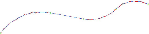
Finding “the right settings” to produce the “ideal solution” often requires some trial and error. If you are not sure which setting will yield your ideal solution, you may want to set up a workspace using the Inspector transformer to show the original linework overlaid with the Curvefitter results.
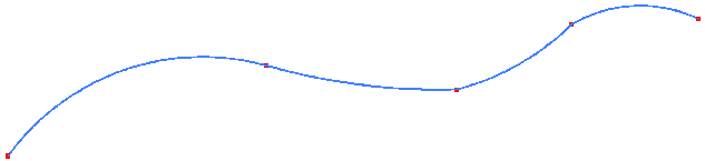
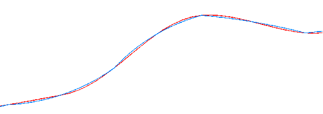
First we try a precision of 0.5 feet
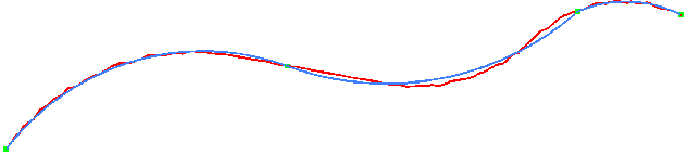
This creates a solution made up of 3 arc segments. Notice that this solution yields a fairly smooth transition between the leftmost segment and the middle segment but the rightmost segment is less smooth – the rightmost two segments are obviously not tangent.
Try a more precise setting
In this situation we may get a more accurate and smoother solution by using a smaller Precision value. This is often the case when accuracy and/or smoothness are the most important aspects of the desired result.
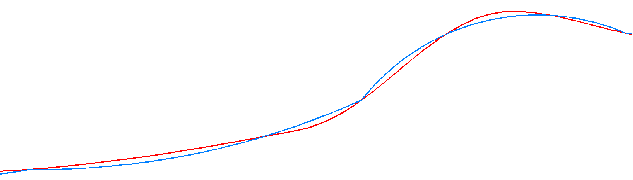
Next we’ll try a Precision of 0.2 feet
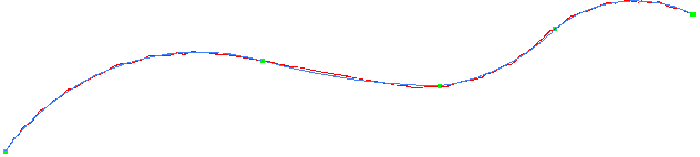
This yields a solution with 4 Arc segments. It fits the original linework more closely and the solution is somewhat smooth but it’s not perfectly smooth.
Unbalanced emphasis
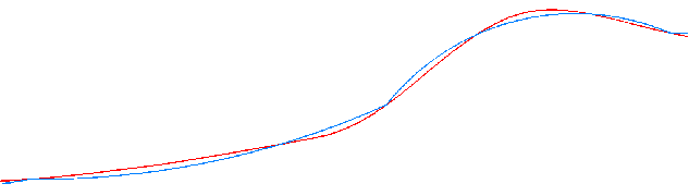
The Curvefitter allows the adjustment of 3 Weights: Compression, Smoothness and Accuracy. Our “ideal solution” is defined as very smooth (because the linework probably originated as engineered segments that were perfectly tangent) and we are not so much interested in maximum vertex reduction, so we can adjust the Curvefitter Emphasis to achieve that goal. We will express our desired ideal solution by emphasizing Smoothness the most, Accuracy somewhat less and compression very little.
Curvefitter Emphasis Settings:
- Precision: 0.2
- Compression: 0.1
- Accuracy: 1.0
- Smoothness: 10
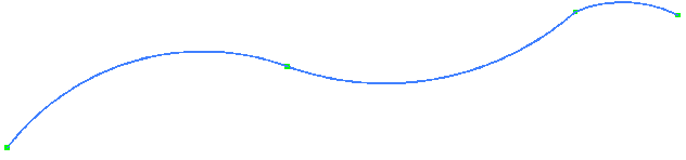
The results – nearly perfect smoothness and still accurate to within 0.2 feet.
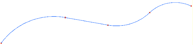
This solution uses 4 segments: an Arc, followed by a straight segment, followed by 2 arc segments (left to right). This is our “Ideal Solution” realized.
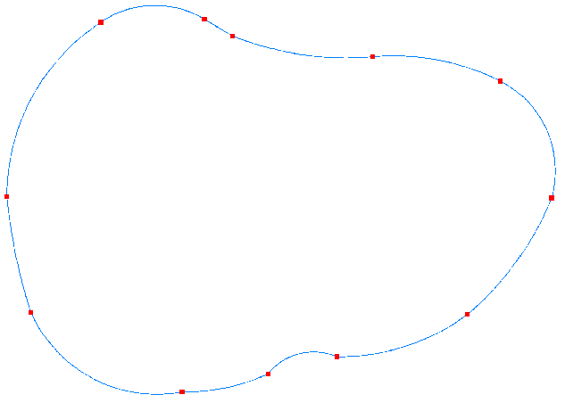
Example 2: This linestring could have been extracted from any FME-supported format. It’s a closed polygon, very smooth and it’s made up of 440 straight line segments.
440 straight segments
Area = 260,909
Our Ideal Solution
In this example, we will assume the goal is to focus on compression and accuracy – with accuracy defined as polygon computed area difference.
A close-up view of the polygon with the vertices highlighted.
Our first guess for Precision will be 1. We will start with Balanced Emphasis and look at the resulting polygon overlaid with the original.
Curvefitter Settings:
- Precision: 1
- Emphasis = Balanced (all set to 1)
- Results
- Vertex Reduction = 1 : 25.88
- Area of CF polygon = 261004
- Area Difference = 0.0364%
We can see that these settings give us more than a 25:1 compression, fairly accurate reproduction of the polygon and a very slight change in area.
More Compression Please
In order to gain a higher compression (more vertex reduction), we will try increasing the Precision (leaving the emphasis balanced for now).
Curvefitter Settings:
- Precision: 2
- Emphasis = Balanced (all set to 1)
- Results
- Vertex Reduction = 1 : 36.66
- Area of CF polygon = 261162
- Area Difference = 0.0969%
This does give us what we wanted with a healthy increase in compression and although the Curvefitter algorithm naturally creates a polygon that tends toward maintaining equal areas, the area of this polygon has a much greater change than the results we saw with a precision of 1.
Since our Ideal Solution for this example is to maintain the polygon area as much as possible and also to achieve a high compression, we will enlist the help of the Curvefitter Emphasis settings.
Curvefitter Settings:
- Precision: 2
- Emphasis
- Accuracy: 10
- Compression: 1.0
- Smoothness: 0.1
- Results
- Vertex Reduction = 1 : 33.84
- Area of CF polygon = 261054
- Area Difference = 0.0555%
With these settings, we fine-tuned the conversion to give us almost the same compression as the balanced emphasis but with a much more accurate area.
Our Ideal Solution has been realized.
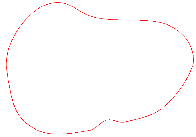
Curvefitter results – 12 segments
11 arc segments and 1 straight segment
Area = 261,05