All features enter the transformer through the Input port.
Restructures and regroups incoming features based on specified “Group by attributes” and calculates summary statistics based on a designated “Attribute To Analyze” in order to form a Pivot table output.
Like its cousin, the StatisticsCalculator, the AttributePivoter groups features according to selected attributes, and computes statistics on a single attribute for all features in each group (Grouping by rows). Beyond this, the AttributePivoter allows for the order of these row grouping attributes to be specified so that a logical nesting of additional summary rows can be generated. In addition, the AttributePivoter also allows for new attributes to be generated dynamically based on the unique values of a selected attribute (Grouping by Column) with values populated by statistics performed on the resultant groupings.
Note: Note: Because the AttributePivoter generates attributes dynamically, you must set any writer feature types to dynamic mode if you want to include these attribute in the output. This is described in more detail in Result Grouping and Tabular Structure.
All features enter the transformer through the Input port.
A single new feature will be output containing all computed statistics for each completely defined row group. The attributes on these features are described in the “Result Grouping and Tabular Structure” section.
The first row emitted from the Data port will contain information to define the schema for a dynamically configured feature type.
For each logically nested grouping as described in the “Result Grouping and Tabular Structure” section, a summary row will be emitted prior to the first data row for the group. It provides summary information for all rows contained in the group. An overview summary of all rows will always be generated.
The first row emitted from the Summary port will contain information to define the schema for a dynamically configured feature type.
One or more attributes are chosen to specify how features are grouped to form the rows of the resulting table. Unlike most “group by” parameters, the user has the opportunity to specify the order of the grouping attributes, so that nested summary groupings can be generated, adding a hierarchical structure to the resulting table.
In addition to row groups, the user can optionally select an attribute whose unique values will generate new attributes, hence “pivoting” the data and further subdividing the groupings on which the statistics are calculated.
A single attribute is chosen upon which to compute statistics. The features are grouped according to the row and column grouping attributes, and statistics are calculated over all values of this attribute within the features in each group.
The user can choose to compute multiple types of summary statistics simultaneously. Each chosen statistic type will be represented as a separate column within each column group of the result table.
One or more of the following statistic types may be selected.
The section entitled “Result Grouping and Tabular Structure” defines a logical nesting of row groups. For each such logically nested group, the AttributePivoter computes summary statistics, which it emits as table rows through the Summary port. The value for the most specific row grouping attribute for the summary row is given a value of “<attrName> <description>”, where <attrName> is the name of the row grouping attribute, and <description> is the value given to the “Row Group Summary Line Description” parameter. For example, if grouping by the attribute “Region_RSS”, the summary row over all regions would have a value of “Region_RSS Total” for the “Region_RSS” attribute, assuming the row group summary line descriptor is left with the default value of “Total”.
Input features are grouped by “grouping attributes”, and statistics are computed on the specified analyzed attribute in each group. There are two kinds of grouping attributes which work together to define these groups:
Because the row grouping attributes are ordered, they effect a sort of logical nesting of groups. At the lowest level, a complete set of unique values is represented as a single row of the result. One level up is the logical grouping consisting of the set of rows where all row grouping attributes are unique except for the last one specified. This logical nesting carries up to the first specified row grouping attributes.
A row resulting from a complete set of unique data values is known as a “data row”. There is an additional “summary row” generated for each logically nested grouping, which summarizes the data for the data rows contained in the grouping.
The sequence of resulting rows form a table with the following attributes:
The first data feature and first summary feature emitted will contain additional attributes which will contain the schema information needed to write the data out to a feature type configured for dynamic writing.
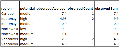
Use AttributePivoter to create a simple pivot table, with the same contents as one created with Excel.
Fictitious data generated in Excel was exported it to a CSV file for use in Workbench. A simple pivot table was also created in Excel to show what we want to produce from FME; basically we want to summarize observed values based on region and potential.
The workspace shown below uses the AttributePivoter transformer to create statistics for the observed attribute, grouping features by region and potential. The new statistics features are written to a CSV file which has all of the same attributes/fields as the Excel pivot table. An additional CSV file is generated to hold the summary for each of the groups in the pivot table. Notice that the output feature types are both defined with dynamic schema; the schema actually comes from the schema information included in the first features emitted from the AttributePivoter’s Data and Summary ports at runtime.

The table written by FME and viewed in Excel resembles the Excel pivot table:
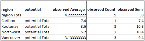
The summary table contains summary information for each group. It has the same schema as the result table above. The “region total” row contains the results for all data within the table.
Using a set of menu options, transformer parameters can be assigned by referencing other elements in the workspace. More advanced functions, such as an advanced editor and an arithmetic editor, are also available in some transformers. To access a menu of these options, click  beside the applicable parameter. For more information, see Transformer Parameter Menu Options.
FME Factory Used: PythonFactory, TestFactory
Search for samples and information about this transformer on the FME Knowledge Center.