FME Form: 2026.1
Raster
|
In this topic: |
|
|---|---|
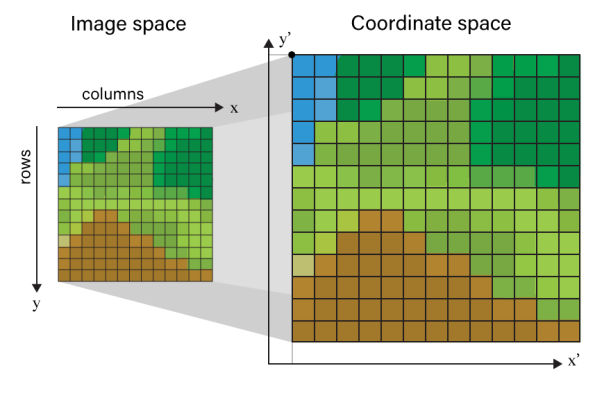
A raster is a rectangular matrix of evenly-spaced cells (sometimes called pixels), arranged in columns and rows.
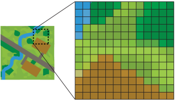
A raster – and therefore its cells – has one or more bands (sometimes called channels or layers). A band’s interpretation determines what range and type of values it can hold.
Each cell has one numeric value per band.
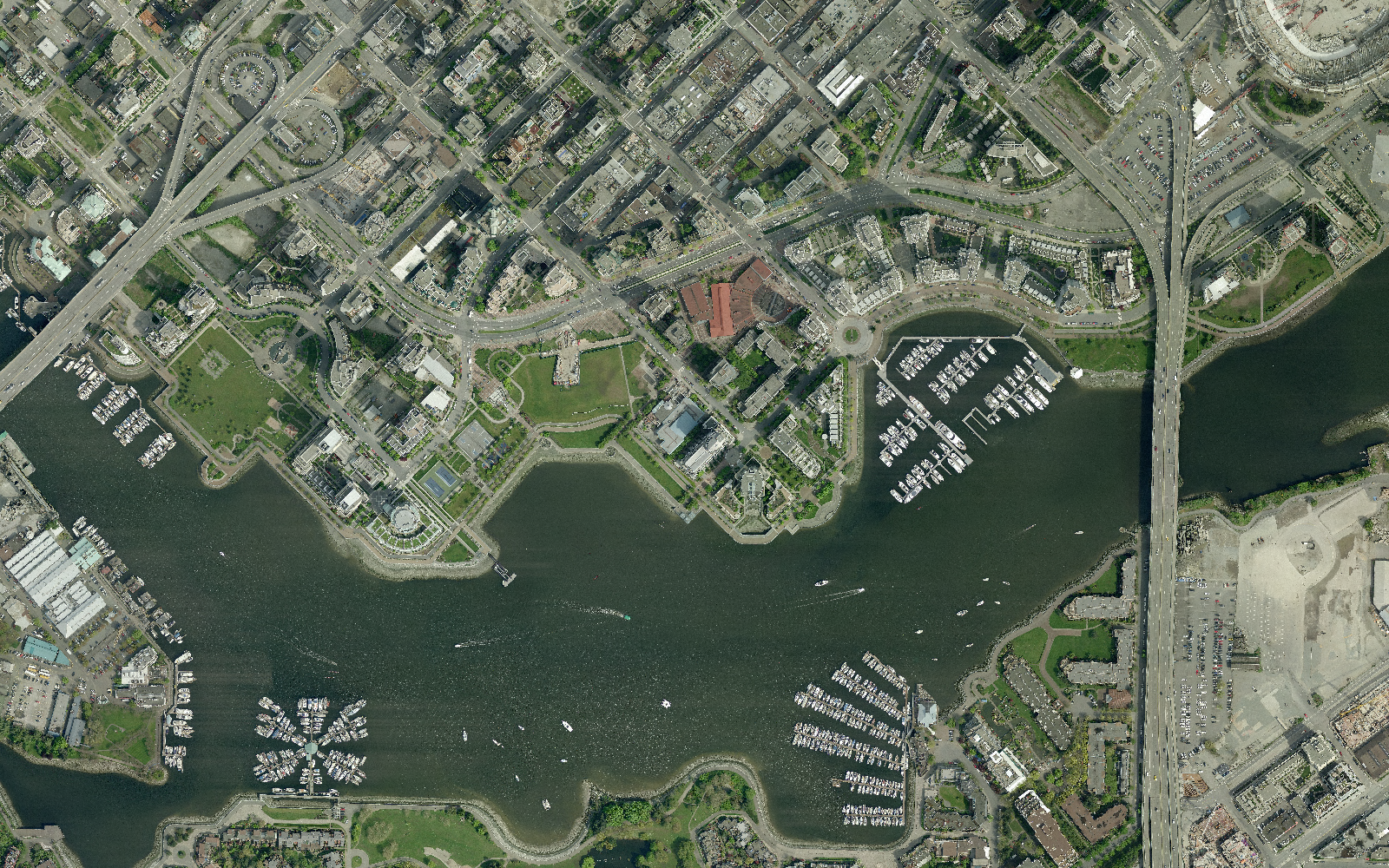
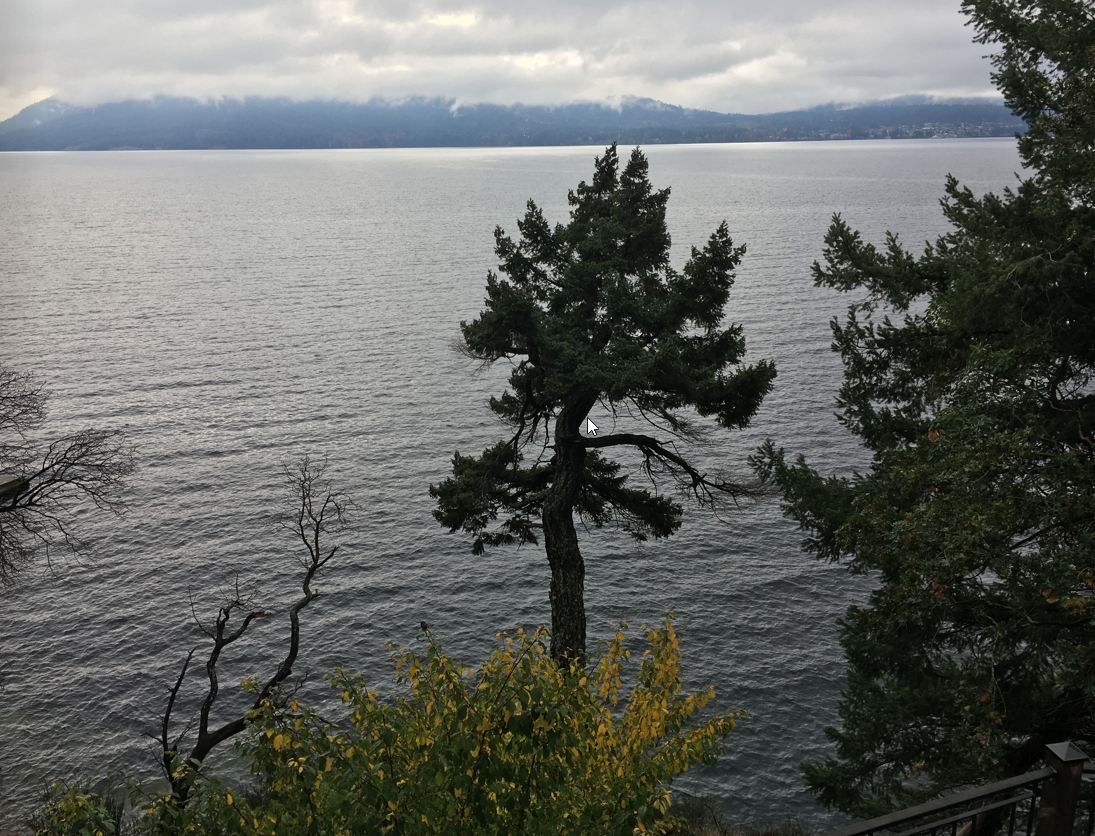
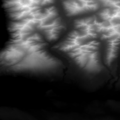
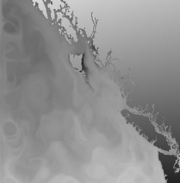
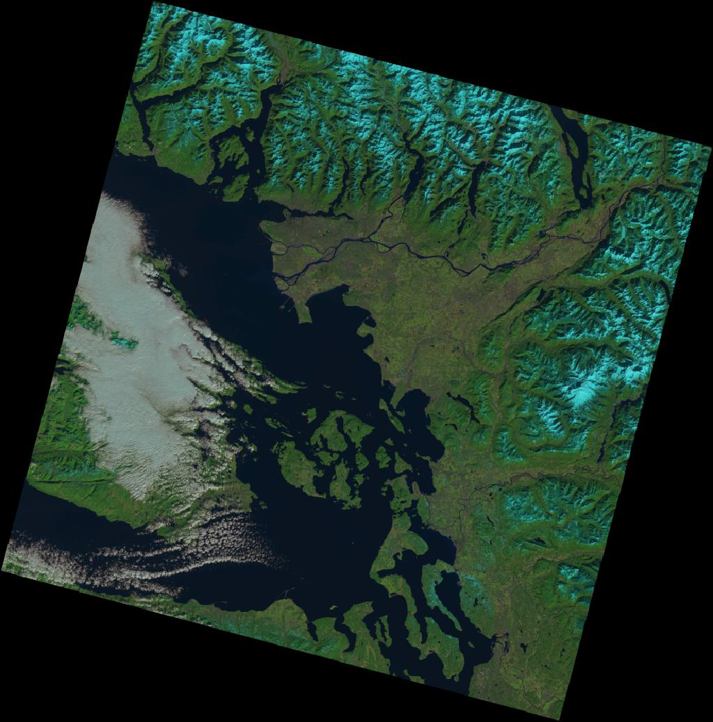
Rasters may represent image or numeric data. Images are commonly derived from satellite data or photography, while numeric data often represents elevations, temperatures, and other quantitative information.
The number of bands will vary – one for a digital elevation model (DEM) or simple numeric raster, three or four for most color image rasters (red, green, blue, and sometimes alpha), and even more for those produced with multiple sensors or representing measurements repeated over time.
|
Orthoimage |
|
|
Photo |
|
|
Digital Elevation Model |
|
|
Numeric |
|
|
Satellite: Multispectral |
|
|
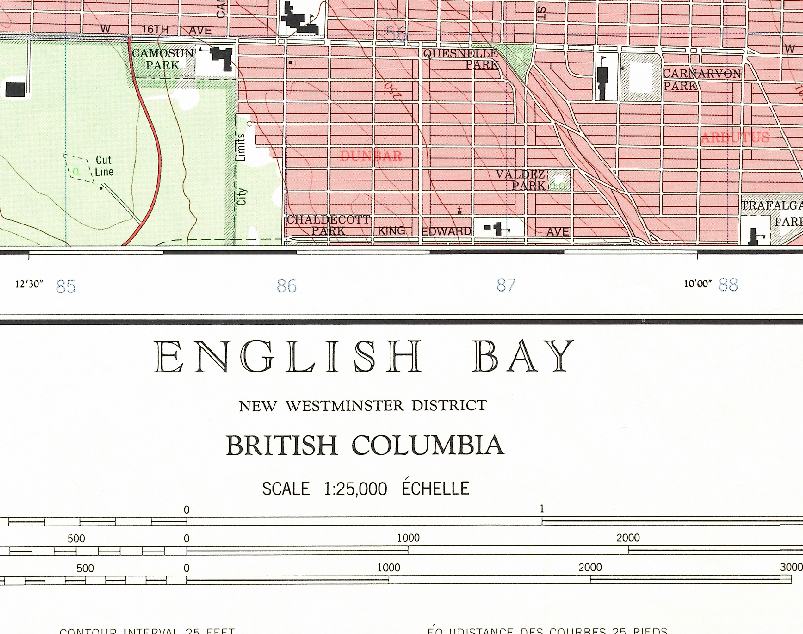
Scanned map |
|
Some rasters are georeferenced, and know where they are positioned on the earth. Some, such as scanned maps, can be manually georeferenced. Some may be tied to a point on the earth (as is a photo with embedded GPS information) but the contents of the image are not georeferenced. Some may be associated with a geographic feature and stored as an attribute, common with scanned documents and images.
Raster Features
In FME, rasters have these attributes and values:
|
fme_geometry |
fme_aggregate |
|
fme_type |
fme_raster |
They will also have a series of attributes that are specific to their format, prefixed appropriately with strings such as geotiff_, pngraster_, cded_, ngrid_, and so on.
Raster Interpretation Types
A raster’s interpretation type reflects its bands’ interpretation types. (See Band Interpretation Type below.)
A single-band raster is described by the same interpretation type as that one band.
A color raster is described as its color and alpha components, along with the sum of bit depths for all bands. An RGB raster with 8-bit bands (Red8, Green8, Blue8) is RGB24. An RGBA (with alpha) with 16-bit bands (Red16, Green16, Blue16, Alpha16) is RGBA64.
Raster Properties
A raster’s origin with regards to its own columns and rows is the upper left corner.
This differs from its geographical extents, which are described from the lower left to upper right corners. If a raster is georeferenced, these corner x and y coordinates will reflect the units of the raster’s coordinate system (meters or degrees, for example).
These properties have a single value per raster, and describe the raster as a whole.
|
Raster Property |
Description |
Sample Values (Orthophoto) |
|---|---|---|
|
Minimum Extents |
X and y coordinates, in ground units, of the lower left corner of the raster. |
|
|
Maximum Extents |
X and y coordinates, in ground units, of the upper right corner of the raster. |
|
|
Resolution (Columns x Rows) |
Total number of columns (x-axis) and rows (y-axis). |
|
|
Origin |
X and y coordinates, in ground units, of the upper left corner of the raster. |
|
|
Spacing |
Fixed distance in the x and y dimensions between each cell in the raster. Some formats store only one spacing value, requiring square cells. Also known as cell size. For georeferenced rasters, spacing is in ground units. |
|
|
Rotation in Radian CCW |
Represents the rotation of a raster relative to the x and y axes. 0,0 means no rotation – the raster is aligned straight along both axes. Rotation is measured in radians, counter-clockwise:
Unequal x and y rotation values will produce a shear. The rotation point is the raster origin (upper left corner). |
|
|
Cell Origin |
The reference point of a cell, that is, the point within each cell from which the pixel for that cell is derived. The lower left corner of the cell in the x or y dimension is The FME default is |
|
|
Affine Transform |
Origin, Spacing, and Rotation form an affine transformation. |
|
|
Number of Bands |
The raster’s number of bands (layers). Minimum is Each band carries one numeric value per cell. |
|
Ground Control Points (GCPs) are sometimes used to georeference rasters. If they exist on a raster, they will appear as a raster property.
Each GCP is a pair of locations, matching a cell (column, row) in the raster to a point in a coordinate system (x,y,z). A minimum of three GCPs are needed for georeferencing.
|
Raster Property |
Description |
Sample Values (Scanned Topographic Map) |
|---|---|---|
|
GCP Coordinate System |
The coordinate system of the referenced points (not necessarily the same coordinate system as the raster). |
|
|
Ground Control Points |
A series of numbered GCPs, starting with zero (0), each consisting of a cell position (column, row) matched to a real-world position (x,y,z) in the designated GCP Coordinate System. |
|
GCPs can either be applied to the raster, resulting in the image being georeferenced and tagged with the GCP Coordinate System, or the GCPs can be extracted and stored on the resulting data file for those formats supporting unreferenced data and GCP storage.
Bands
Rasters have bands – at least one, often more.
A band is a layer of numeric values that spans the entire raster, one value per cell. A band’s interpretation type determines what those values can be, and in some cases, what they mean.
Band Interpretation Type
A band’s interpretation type describes what values it can hold. It consists of type and bit depth.
|
Type |
Name |
Description |
|---|---|---|
|
Int |
Integer |
Whole numbers. |
|
UInt |
Unsigned Integer |
Whole numbers greater than or equal to zero (0). |
|
Real |
Real Number |
Floating point numbers (decimals). |
|
Red |
Red |
The red band of an RGB image. Values are unsigned integers. |
|
Green |
Green |
The green band of an RGB image. Values are unsigned integers. |
|
Blue |
Blue |
The blue band of an RGB image. Values are unsigned integers. |
|
Alpha |
Alpha (Transparency) |
Transparency, used in conjunction with other bands (often RGB or Grayscale images). Values are unsigned integers. Alpha is not Nodata, but can be used to represent areas of no data and make them transparent. |
|
Gray |
Grayscale |
A single band indicating levels of gray ranging from white to black. Typically used for grayscale images. Values are unsigned integers. |
A band’s bit depth determines the range of values that can be used. Higher bit depth means more space to store numbers, which means a wider range of values can be used.
|
Type(s) |
Common Bit Depths |
Value Range |
|---|---|---|
|
Int |
8 16 32 64 |
|
|
UInt |
8 16 32 64 |
|
|
Real |
32 64 |
|
|
Red
|
8 16 |
|
Color
Raster colors are commonly represented by their red, green, and blue components, each on a separate band.
If the color bands are 8-bit, they each will accept values from 0 to 255, and together produce an RGB24 raster, with over 16 million possible colors (256 x 256 x 256).
Numerous other color spaces exist (that is, methods of representing color) such as CMYK, HSV, YrCbCr and more. These may be supported by some raster formats, and may be converted to RGB on read or write. Note that a color space conversion is generally lossy.
|
|
Red8 |
Green8 |
Blue8 |
|---|---|---|---|
|
White |
255 |
255 |
255 |
|
Black |
0 |
0 |
0 |
|
50% Gray |
127 |
127 |
127 |
|
Red |
255 |
0 |
0 |
|
Green |
0 |
255 |
0 |
|
Blue |
0 |
0 |
255 |
Alpha and Nodata
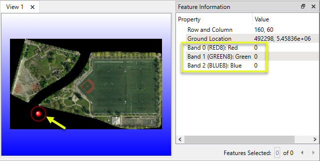
Alpha bands are often used with RGB rasters, forming RGBA. The alpha value indicates transparency, where zero (0) is fully transparent and the maximum value (255 if 8-bit) is fully opaque. This affects the display of the other bands, and is often used to create transparency where no data exists, as in irregularly shaped or rotated rasters which might otherwise have areas displayed as black pixels.
In this example, an irregularly-shaped raster is produced by clipping to a park boundary. Cells that fall outside the park boundary but inside the raster's rectangular extents are black.
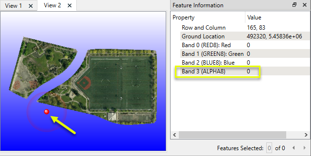
By adding an Alpha band with the value zero (0) in locations that have no data, they are rendered as transparent.
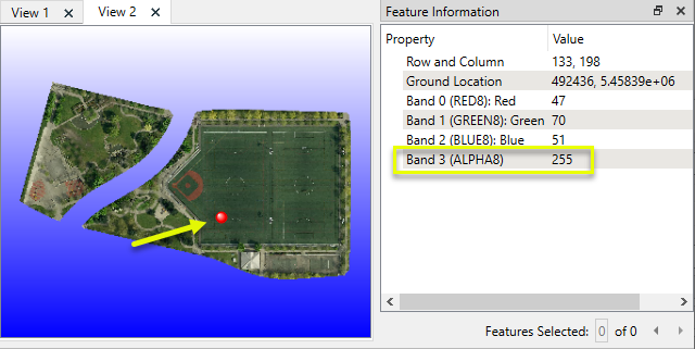
Note that pixels in the Alpha band in locations where there is data – that is, color – have a value of 255, which is fully opaque.
Nodata is a designated value, per band, that is specified to mean no data – unknown or invalid, as opposed to null or zero.
Nodata is frequently displayed as transparent, but alpha and Nodata are not the same. In general, Nodata is useful for gridded numeric datasets, while alpha is useful for color rasters.
Nodata can also be used in the context of raster palettes – see below.
Not all raster formats support Nodata.
Another option for identifying unknown or invalid data is a separate band that acts as a flag for each cell, indicating whether the data is valid or not.
Nodata Values
Consider the following when selecting Nodata values or performing operations that change cell values:
-
The Nodata value must be valid for the band interpretation type – that is, fall within the range of acceptable values. For example,
-1is a valid Nodata choice for an Int8 band, but not a UInt8 band. -
NaN (not a number) is a valid floating point value for Real bands only.
-
-32768 is often used for Int16 bands, as the minimum value for that type.
-
Because the Nodata value falls within the acceptable range of values for a band, it is possible to inadvertently mark cells as Nodata (or the inverse) when performing operations that change cell values. Similarly, assigning a new Nodata value to a raster has the risk of marking valid cells as Nodata.
-
Zero (0) might seem a good choice for Nodata, but color rasters use zeros to represent black. An alpha band may be better when working with RGB/RGBA images.
Band Properties
Band properties describe one band on a raster. They can include:
|
Name |
Bands are numbered, starting at zero, and referred to as Band 0, Band 1, Band 2, and so on. The Name property optionally stores an additional name for the band, often used to descriptively name Red, Green, Blue, and Alpha bands for color rasters. |
|
Interpretation |
Data type and bit depth of the band. See Band Interpretation Type above. |
|
Number of Rows Per Tile
|
Rasters may have internal structures optimized for different storage and access methods. A cloud-optimized format might store it in 256 by 256 pixel tiles, where another format may store it in horizontal strips that are full raster width by 1 row in height. These values are not generally useful to users. For the entire raster’s size, see Raster Properties > Resolution (Columns x Rows). |
|
Nodata Value |
An optional cell value that represents invalid, unknown, or non-existent data. |
|
Number of Palettes |
If a band has one or more palettes, this property will contain the total number. |
Interleaving
Interleaving is the manner in which cell values are organized for binary storage. These are common methods for multiband rasters:
|
BIL |
Band Interleaved by Line |
Stores values band by band, per row. RRRRGGGGBBBB |
|
BIP |
Band Interleaved by Pixel |
Stores values band by band, per pixel. RGBRGBRGBRGB
|
|
BSQ |
Band Sequential |
Stores values by band. RRRR
|
|
Tiled BSQ |
Tiled Band Sequential (Cloud Optimized) |
A variation of BSQ in which values are stored by band, within tiles optimized for efficient streaming retrieval. RRRR
|
Internally, FME uses BSQ for bands and BIP for palettes.
Palettes
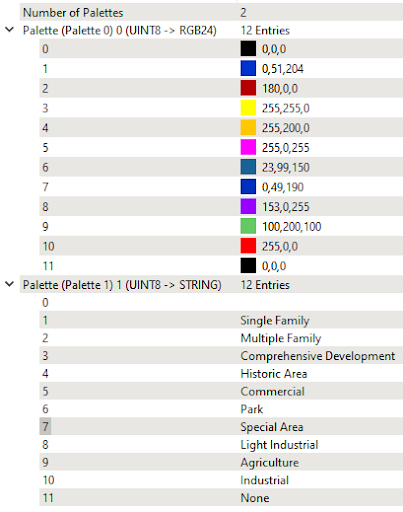
A palette is a lookup table (LUT), correlating a cell’s value with something else. That something else might be an RGB color, a word, or other value.
A palette is associated with a specific band. A band may have zero, one, or multiple palettes. Palettes can serve a number of purposes:
-
Reduce file size by paletting a color image, reducing three bands (R,G,B) to a single numeric band
-
Reducing file size or complexity of a raster by limiting the number of available values
-
Providing one or more thematic interpretations of a gridded dataset by applying colors or strings – often both, as in the color blue and the string
Water. -
Providing descriptive names for values
Rasters with palettes are sometimes referred to as classified rasters.
The palette consists of a series of pairs of palette keys and palette values. The palette key is matched to the band’s cell values, and must have the same interpretation type as the band. Bands must be a UInt8, UInt16, or UInt32 interpretation type to have palettes. Palette keys of UInt64 are not supported.
Palette values can be RGB24, RGBA32, RGB48, RGBA64, Gray8, Gray16, or String, as in this example:
Palette Properties
Palette properties describe one palette on one band of a raster.
|
Property |
Description |
|---|---|
|
Name |
Palettes are numbered, starting at zero, and referred to as Palette 0, Palette 1, Palette 2, and so on. The Name property optionally stores an additional name for the palette. |
|
Key Interpretation |
The interpretation type of both the related raster band and the key correlation values. |
|
Value Interpretation |
The interpretation type of the referenced value, such as an RGB color or descriptive string. |
Palettes and Nodata
Palettes do not directly store Nodata values.
However, since the palette keys are intended to match the band values, a single palette key can be interpreted as Nodata if it matches the band’s Nodata value. This Nodata key also looks up to a palette value, which is then considered the Nodata value.
Removing and Resolving Palettes
Palettes can either be simply removed from a band, leaving the original cell values intact, or they can be resolved – that is, have the palette values overwrite the cell values.
If the palette values are RGB(A) colors, multiple bands are created to hold each component value.
The resulting bands will have their interpretation type adjusted to match the resolved palette values if necessary. The palette is removed.
String palettes cannot be resolved.
World and TAB Files
Both world files and TAB files are sidecar text files – ancillary files that carry additional information about a raster when necessary.
World files contain only georeferencing affine transformation values, whereas TAB files may contain control points, coordinate system, and sometimes user attributes.
Readers that read both world and TAB files give precedence to the world file for georeferencing.
World Files
World files contain raster georeferencing information by way of an affine transformation, that is, x and y values for origin, spacing, and rotation (skew).The file name will match the corresponding raster, while the file extension varies between formats, but generally contains the letter w such as WLD, TFW, and BQW.
Some raster format readers will read world files present alongside a dataset, and many raster writers have the option to generate a world file to accompany the output dataset.
If different georeferencing values are provided in the world file versus the raster, the world file takes precedence over the internal raster values.
Most raster format writers will not create a world file if the output raster contains only default georeferencing information: an origin of (0, 0), spacing of 1.0, and rotation of 0.0.
Refer to specific format reader/writer documentation for details of world file support.
TAB Files
TAB files contain raster georeferencing information by way of control points and a coordinate system definition. User attributes are sometimes stored here as well.
Control points pair individual cells with real-world coordinates, and can represent the raster’s extents (corners) or specified Ground Control Points.
Most raster format readers will read TAB files present alongside a raster dataset, and most raster format writers have an option to generate a TAB file to accompany the output dataset.
Attributes are not generally a part of raster TAB files. However, FME will read and write attributes to raster TAB files in the same manner as it does for vector TAB files. This enables the storage of user attributes for many formats that do not otherwise support attribution. To determine whether a raster format can store user attribute information via TAB files, see User-Defined Attributes in the specific format reader/writer documentation.
If different georeferencing values are provided in the TAB file versus the raster, the TAB file takes precedence over the internal raster values.
Refer to specific format reader/writer documentation for details of TAB file support.
Raster Processing
FME has a selection of transformers for processing rasters.
FME features with raster geometry cannot be processed in all the ways that vector features can. If an unsupported operation for a raster is attempted, a vector FME polygon feature is used instead. This substitute feature represents the original raster bounding box, and contains the original attributes.
Band and Palette Selection
FME transformers that support band and/or palette selection are able to operate on chosen bands and palettes, rather than the entire raster (all bands and palettes).
The default state of a raster is all bands and all palettes selected. To change that, use a RasterSelector to specify which bands and/or palettes are to be active and selected. Subsequent transformers will operate on those chosen bands and/or palettes only until the selection is changed.
Use another RasterSelector to re-select all bands and palettes to return to the default state.
Bands and palettes are numbered, starting at zero, and are selected by their number(s).
Tiling and Mosaicking
A raster can be tiled into a series of smaller adjacent rasters, and multiple adjacent rasters can be mosaicked into one larger raster.
Band Combining and Separating
Band combining is not mosaicking – it is the creation of a multi-band raster by stacking multiple rasters that have identical extents and resolution into a single raster. All bands retain their values, unaltered.
Examples include assembling an RGB raster from three individual red, green, and blue band rasters, or generating a scientific gridded dataset with recurring measurements over a time period.
Band separating is the inverse operation – creating one raster per band and/or palette of a multi-band (or multi-palette) raster. A common use is writing multi-band or multi-palette rasters to formats that support only single-band or single-palette output.
Pyramiding
Pyramids are downsampled (lower resolution) versions of a raster, sometimes referred to as overviews or thumbnails. They are usually generated to improve performance, and are particularly useful for web streaming rasters.
When zooming in and out, cached pyramids can display more quickly than resampling the raster at each zoom request.
Compression
Rasters can be rather large in terms of storage space.
A variety of methods exist to compress rasters, reducing their size. These algorithms fall under two categories:
-
Lossless – compresses the raster while preserving its original cell values. Examples include:
-
Runlength coding
-
Blockwise coding
-
Quadtree coding
-
Huffman coding
-
LZ77
-
-
Lossy – compresses the raster with some generalization of cell values, typically in color variation not noticeable by the human eye. Examples include:
-
Discrete Cosine Transform (DCT) – such as JPEG
-
Wavelet compression – such as JPEG 2000
-
Lossy methods can usually produce higher compression ratios than lossless.
Raster size can also be reduced by reducing resolution (downsampling) to increase cell size, or by paletting, which reduces and generalizes values to a limited set. Both of these methods are lossy.
Raster File Naming
FME features with raster geometry each typically represent one raster data file, though some raster format datasets such as GeoTIFF can contain multiple images.
Raster writers typically accept a folder as a destination dataset.
When writing multiple raster files for one dataset folder, the feature type name is used to determine the filename. If multiple features are written to the same dataset, the name will be suffixed to be unique.
Most file-based raster format writers fan out on fme_basename. The feature type will be the value of the fme_basename attribute, which is set by all raster format readers to be the filename, without path or extension.
For example, on reading the two files image1.tif and image2.tif, two features would be produced- one with an fme_basename value of image1, and one with a value of image2. If these two features were then sent to a PNG writer fanning out on fme_basename, two new files would be produced – image1.png and image2.png.
Raster format writers that store their data in files avoid overwriting existing files and differentiate output files from one another when multiple rasters are written (particularly if the writer outputs one file per raster feature). A simple renaming mechanism prevents name collisions. The first output file is written using the name requested in the workspace. Additional files are automatically distinguished by appending sequential numbers to the filenames. For example, if four rasters are written to the same feature type, named image, the result is a set of output files with the names image.tif, image_1.tif, image_2.tif, and image_3.tif.
Note that renaming the output files only occurs within a single instance of the writer within a given translation. Multiple translations of the same workspace that incorporates a file-based raster writer will overwrite previous file output if name collisions occur. Similarly, using multiple writer instances targeted at the same folder is considered unsafe if the same feature types are used in both translations, as overwriting may occur.